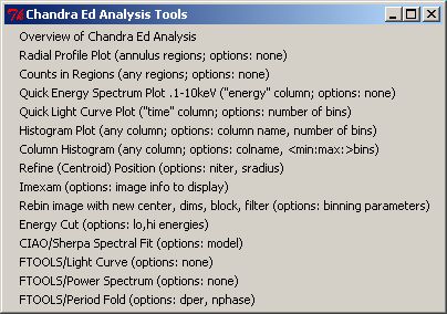
Part 3: First Look at Quantitative Analysis using ds9
Spatial Analysis
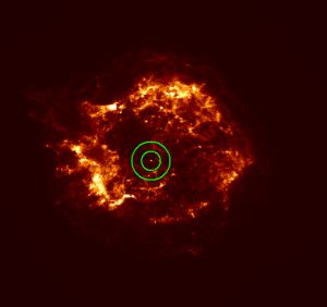
We are now going to run some programs on our region of interest which will give us a quantitative result. To use these programs you must have defined a single circle region of interest at the position X,Y 4158,4398 (as described in the last section.) The Counts in Regions and Radial Profile Plot perform analysis on the position information of each detected X-ray photon. They essentially count up the number of X-ray photons within a given spatial region and give you visual output that allows you to compare results.
The analysis we want to run first is called Counts in Regions. The program sums up the X-ray photons in the region(s) specified.
To run this program:
Pull down the Analysis menu and select the menu option Counts in Regions.
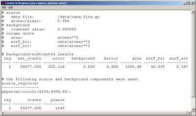
In a few seconds, a window will display your analysis results.
The net_counts value is the number of X-ray events inside the region.
The surf_bri (surface brightness) value is a measure of the average number of X-ray photons in a unit area
Read a more detailed discussion of what this kind of analysis means, and an exercise.
Now move the region around to different places on the Cas-A image and run Counts in Regions in different locations. Doing this will give you a quantitative idea of how strong the X-ray emission is in various parts of the image.
When you finish, delete the circular region by pulling down the Region menu and selecting the Delete All menu option. Alternatively, you can put the mouse inside the region and press the Delete key.
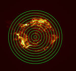
To get a better idea of the shape of X-ray emission from interesting parts of Cas-A, we can run another program on our regions of interest called a Radial Profile Plot. This program will display a graphical plot of the brightness of the X-ray emission (average number of photons per unit area) in concentric annuli around a central point.
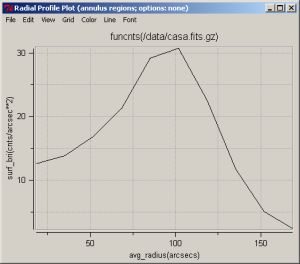
If the X-ray emission in our region is coming from a very strong central source, the shape of the plot will fall off steeply.
If the X-ray emission is less strong (but still coming from a central source), the plot will have a more gradual downward slope.
If the X-ray emission comes from a diffuse source, the plot might not even have a recognizable shape.
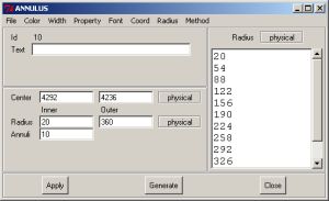
Creating Annuli Regions
Because the radial profile program plots the brightness at defined points moving outward from the center of the region, the radial profile plot runs on a different kind of region of interest, the circular annuli. To create a radial profile plot we must create an annulus region instead of a single circle.
Again, for this exercise, choose the area of the Cas-A image where X,Y equal 4158,4398.
Pull down the Region menu, select the Shape sub-menu.
In the Shape sub-menu, choose the Annulus sub-menu option.
Create an annular region by moving the mouse to the location on the image where you want to place the region and click the left mouse button.
By default, an annulus region with 2 annuli will be displayed.
Having created an annulus region, we now can run Radial Profile Plot.
Pull down the Analysis menu and select the Radial Profile Plot menu option.
In a few seconds, a plot window will display your analysis results.
Try running this analysis program on annuli in different places on the Cas-A image by moving the annulus. For example, move it to near Physical X,Y = 4506,4576 (in the "empty" part of the image). See how the resulting radial profile is much different from that of the bright area at X,Y = 4158,4398.
When you have finished, pull down the Region menu and select Delete All to remove the annulus region.