Part 3: First Look at Quantitative Analysis using ds9
Spectral Analysis
With Counts in Region and Radial Profile Plot we performed analyses on the position information of the photons. Now we want to perform analysis on the spectral (energy) and timing information associated with the X-ray photons that Chandra detected from Cas A. Learning about the energy characteristics of X-ray emission is an extremely important part of the science we can get from this Chandra observation. These characteristics can tell us much about the material composition of the object, as well as the physical processes that it is undergoing.
The first step in spectral analysis is to extract the energy information in the form of a spectrum.
A spectrum is a one dimensional histogram of the number of X-ray photons falling into each of the discrete energy ranges (or bins) that the Chandra detector (ACIS) can identify.
We usually do this within a single circular region of interest, just as we did for spatial analysis with the Counts in Regions task. Before you start, be sure that you have deleted any other regions created prior to this exercise. And, since the region shape was changed to "annulus" in the last exercise, you must change it back to "circle" for this activity.
Create a circular region. Since the region menu will retain the last shape used, which was the annulus, we cannot just click on the image to create the circle. First, you must use either the Shape sub-menu of the Region menu or the region tool bar to set the shape back to "circle". Then move the cursor in the image to the area on which you want to center the region and click the left mouse button.
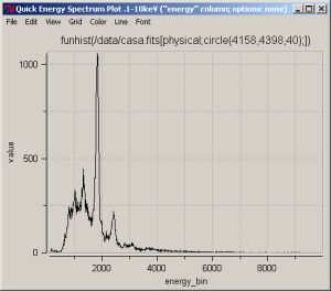
Create a region at the bright area X,Y = 4158,4398, pull down the analysis menu and run the Energy Spectrum Plot.
Move the region and run the Energy Spectrum plot at other areas around the image. Notice how the spectrum changes! What you are seeing is that different elements are present in different regions of the supernova remnant. How this happens and what it means are interesting questions that scientists are currently addressing.
Time Intervals for Plots
The Chandra data set you are using is an ACIS observation and has a binning time of 3.24104 seconds. Any photon that is detected within that interval will be assigned the same arrival time. We therefore must decide how to divide up our data. We can choose to do this in a number of ways. The most informative is to choose a bin width that has a reasonable number of photons in it, and to normalize it as a function of time, so that we can see the count rate, i.e. the number of counts each second that the satellite detects. For now, you can enter 32.4104 seconds. This means that each point on your graph that you will be plotting contains all the photons recorded from 10 timing intervals during the observation.
Timing Analysis
A similar analysis can be made of the timing information associated with each X-ray photon. Once again, we perform the analysis in circular regions of interest. This time, however, we extract timing information from the data in the form of a light curve.
A light curve is a one-dimensional histogram of the number of X-ray photons that fall into discrete time bins.
Plotting a Light Curve
Select a circular region by clicking on the Cas A image. (You can do this by clicking directly on the image because "circle" is still the selected shape in the Region menu.) Again, you can start with the bright area X,Y = 4158,4398.
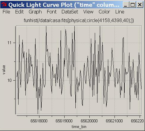
Go to the Analysis menu and click on the option Light Curve.
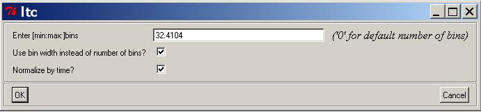
When you select this task, a dialog box will pop up asking you to enter the number of bins to use. Specifying the number of bins is necessary because the timing information recorded by ACIS and HRC is not continuous, but has values that get read out by the instrument in discrete intervals.
Enter a binning time of 32.4104 seconds in the top line of the dialog box, and check both boxes in the two subsequent lines. The value 32.4104 is the binning time of the observation multiplied by 10 so that there are enough photons in each bin to give us a count rate we can see.
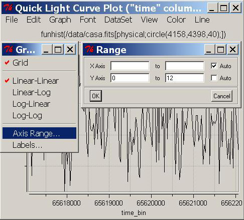
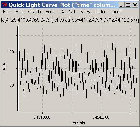
Notice that the light curve seems to be changing. But looks can be deceiving. Look at the values on the y-axis. You are not seeing the whole picture here. If you click on Graph-->axis range... and change the Y-axis plot to read from 0 to 12, and then unclick "auto", you will see something that looks like this!
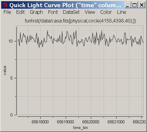
Then, we you click OK, this is the graph that emerges:
So you see that the light curve (or intensity of X-ray energy) is virtually constant; it doesn't change as time goes on. Later on, you will see objects that have extremely interesting light curves; entire stars, that appear to spin around many times in one second! To whet your appetite, here is a light curve from one of the activities you can find on this site, entitled:
"Clocks in the Sky".
Here we see an object whose intensity changes by a tremendous amount over a period of about 4.8 seconds. Just like a lighthouse beams its radiation as it rotates, this X-ray star, Cen X-3, spins on its axis with a precision better than even a Rolex watch, and we can measure this variation with Chandra. Amazingly, by tracking these changes, we can tell what type of object this star is, deduce that it is a member of a double star system, and determine exactly how big the whole system is.
The activities and exercises in these sections were designed to familiarize you with the features and controls of the ds9 imaging system, and the functions that exist on the analysis menu. We have concentrated on what you are doing, not really why you are doing it. You should repeat these activities and exercises and invent some of your own until you are comfortable using ds9. Then you can use the Activities and Images section to focus on the science content and find out more about the fascinating objects that exist in the X-ray universe.